Introduction

There are a lot of great articles and blog posts about Twitter Sentiment Analysis and Classification using all sorts of open-source libraries like Tensorflow, PyTorch, etc. However, In production enviorment where time is of utmost importance, one cannot invest too much time in designing model architecture and fine-tuning it to precision. In such cases (like hackathons, for example), fastai can be used. Basically, this library simplifies training fast and accurate neural nets using best practices.

The Data

Twitter US Airline Sentiment dataset can be downloaded from here.

The data was scraped from February of 2015 and contributors were asked to first classify positive, negative, and neutral tweets, followed by categorizing negative reasons (such as “late flight” or “rude service”).

Although the data has 15 columns, most of them aren’t really of much use since they are either not correlated to the target or have too many NULL values in them which makes it very hard to impute them.

For the sake of easy implementation, we only choose 2 columns, the text column and the airline_sentiment column.

• text: The raw text of the tweet
• airline_sentiment: This is the target label. It has 3 possible values: neutral, positive and negative

As you can see, this is a 3-way classification problem in NLP. Personally, I haven’t found a lot of text datasets with 3-target labels which makes this a good practice problem to work on.

Let’s take a look at the raw data now;

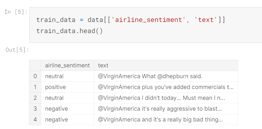
The text column of the data is very much raw at this point. You can observe the @ tags and other things.

Also, since we are using text and airline_sentiment columns, there is no null values in the dataset anymore. There are ~14K samples in the dataset.

Data Visualization

Now that we know how our raw dataset looks like, let us start our Exploratory Data Analysis.

Target Value Distribution

As we noted above, the target column, airline_sentiment (which we have to predict) has 3 possible values. Let us see how these 3 values are distributed.

As seen from the above Pie chart, we can observe the following:

• ~63% of tweets belong to Negative category, which is normal if you think about it since mostly the users will take it to twitter to tweet about their airlines only when they have faced problems during their flight or otherwise.
• ~21% of tweets are Neutral. One thing to note here is that, some of these neutral tweets would probably be negative but in a very subtle sense which would’ve caused them to be wrongly classified as neutral.
• ~16% of tweets are Positive.

Character Frequency Count

Now let’s see the count chart of character frequencies in the tweets. Note that we are talking about individual characters and not whole words.

If you look at all 3 plots carefully, you will notice that the average character frequency for Negative Tweets is much higher than for both positive and neutral tweets (in-fact, both of them combined!).

Any guess for why that might be?

Well it’s simple, If I am “genuinely” angry at an airlines about some problem that I have faced, then I would go on writing large sentences about details on the problems, etc.

Note that an angry client would also tag multiple accounts (like for example the CEO of that airlines and the head of the avaition dept, etc) which would further increase the tweet length significantly.

Word Frequency Count

As we noted from above that the average number of characters would be greater in negative tweets, this logic applies to individual words too (since, more characters = more words).

We can now observe the same pattern as the character frequency count above.

Average Word Length Distribution

Now, let us average word length for each category.

As seen from the distribution above, the average word length for negative tweets is greater than both positive and negative categories.

Unique Word Count Distribution

Let’s see the presence of unique words in each category.

More unique words are present in Negative tweets, followed by Neutral and then Positive tweets.

Word Cloud

Finally, let’s see the Word Clouds for all 3 categories.

Data Preprocessing

Now that the EDA is over, let’s now pre-process the data to make it suitable for modelling.

Note: I am not showing the actual code here. You can look at the Colab Notebook or the Kaggle Notebook for the Complete Code.

Here are the steps that I went through to clean the dataset:

• Removed URLs, @tags and other dirty bits
• Loaded stopwords (from nltk module) and removed stopwords from the dataset
• Converted the text to lower case
• Renamed the airline_sentiment column to label for easier operations
• Changed the “positive”, “negative” and “neutral” to numbers for training. (“negative” -> 0, “positive” -> 1, “neutral” ->2)
• Split the dataset into training and validation split after shuffling the data (15% data goes in validation set).

Data Modelling

Now that the data is cleaned, I am going to use Unified Language Model Fine Tuning (ULMFiT) to train the model. Read more about it here.

Preparing Data for Modelling

Since we currently have raw data in our hands (although cleaned but it still is a pandas dataframe). If you have done Natural Language Processing with PyTorch, you will find this very familiar (I ditched tensorflow 2 a week ago).

Now will create a Data Bunch using the TextLMDataBunch class (think of it as a Wrapper around your dataset). We’ll also create a Data Classifier using the TextClasDataBunch class (this one is used for classfying) 1.

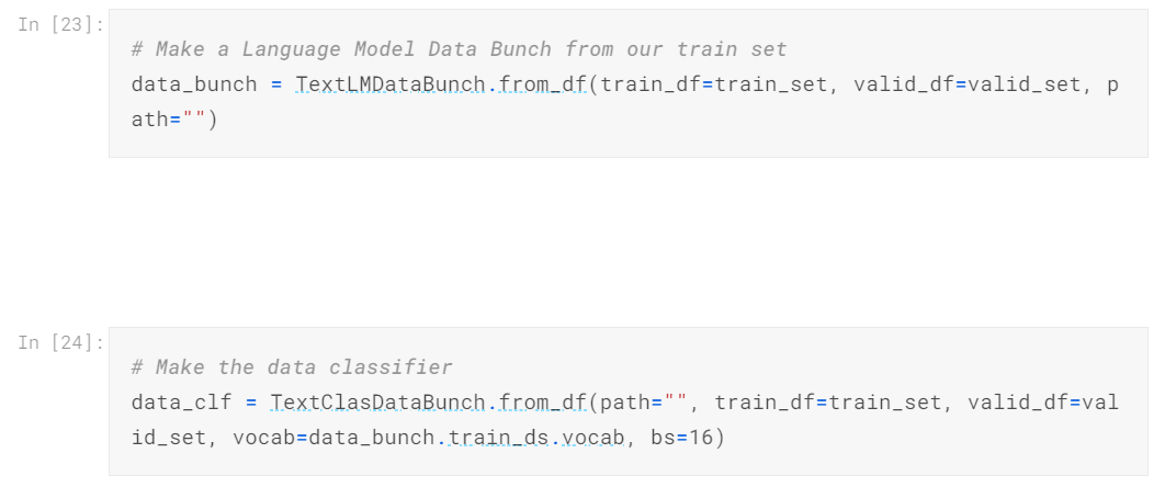
Our model is now ready for training! Yes, we wrote like 2 lines of code and our model is ready of training.

Training the Model

FastAI provides many utilities to train your model but since the general training task is now easier, our time and efforts must be invested more into hyper-parameter tuning and other fine-tuning techniques to get the most optimal results.

Vanilla Training - Language Model

Let’s first train our model straight away without doing any effort to see the baseline we get.

In this, we will first make a language_model_learner with parameters (see the image below) and then fit it for 1 Cycle.

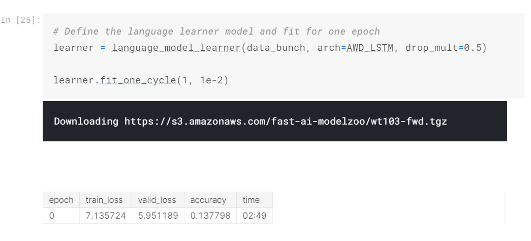
As you can see, the accuracy isn’t very good. But this isn’t our classifier. This is used to learn from the dataset we provided. However, if the learner’s accuracy is increased, then so will the classifier’s accuracy. 2

Partial Unfreezing - Language Model

The model we are using for training consists of LSTM layers internally. FastAI gives us the ability to freeze or unfreeze a certain number of layers.

What does that mean? Well, when we train our model, we are not changing the weights of the layers in the model (since the loaded model is already trained on a lot of data). Such model layers are called “Freezed”. Their weights don’t get updated in Backpropagation.

When we unfreeze those layers, we allow them to learn through the data.

Below, we unfreeze last 3 layers and then see their results respectively.

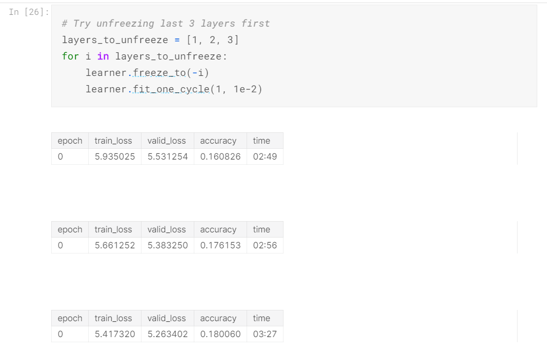
As you can see, model’s accuracy increases with unfreezing more and more layers.

Complete Unfreezing - Language Model

Let’s now see what happens when we completely unfreeze all the layers in the model.

Now, all the layers in the model will be trained on the data.

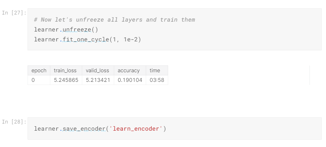
The model accuracy hasn’t improved much further than 19%. It is most likely the maximum it is for now.

We have also saved our model (which is basically just the encoder, so that we can load it for our classifier).

Training the Classifier and Unfreezing all layers

Now that our learner has achieved an OK accuracy, let’s now train our classifier to classify sentiments.

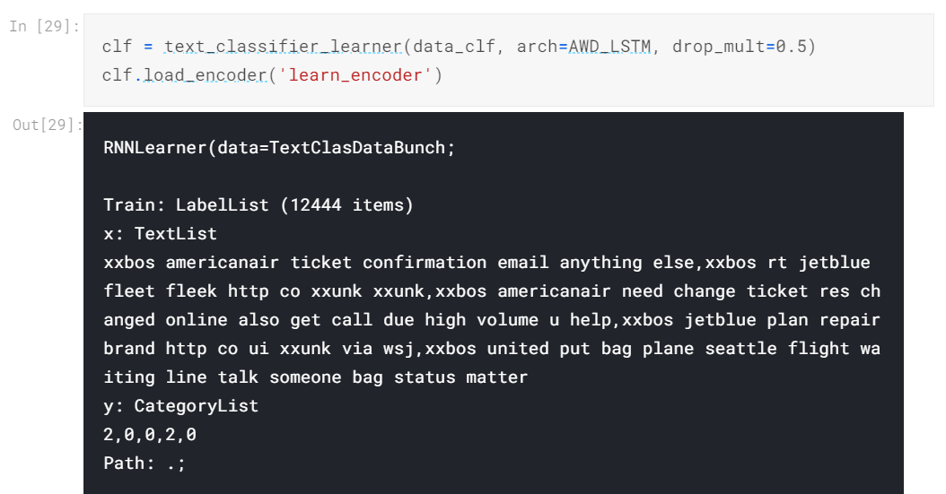
After some previous experimentations with it, I have found that partial unfreezing doesn’t produce good results with the classifier and so we will directly unfreeze all the layers at once after training it without unfreezing.

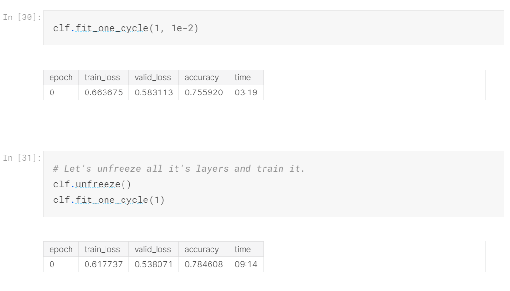
As you can see we have achieved an accuracy of 78%.

Discriminative Fine Tuning - Classifier

This is the last fine tuning technique I have to offer. I will skip the maths and other details, if you want to see a detailed implementation, visit this.

The essence of DFT is that, since we have multiple layers with varying depths, it makes sense to use different learning rates for different layers in the model. For this, I have used the slice() function, about which you can learn more here.

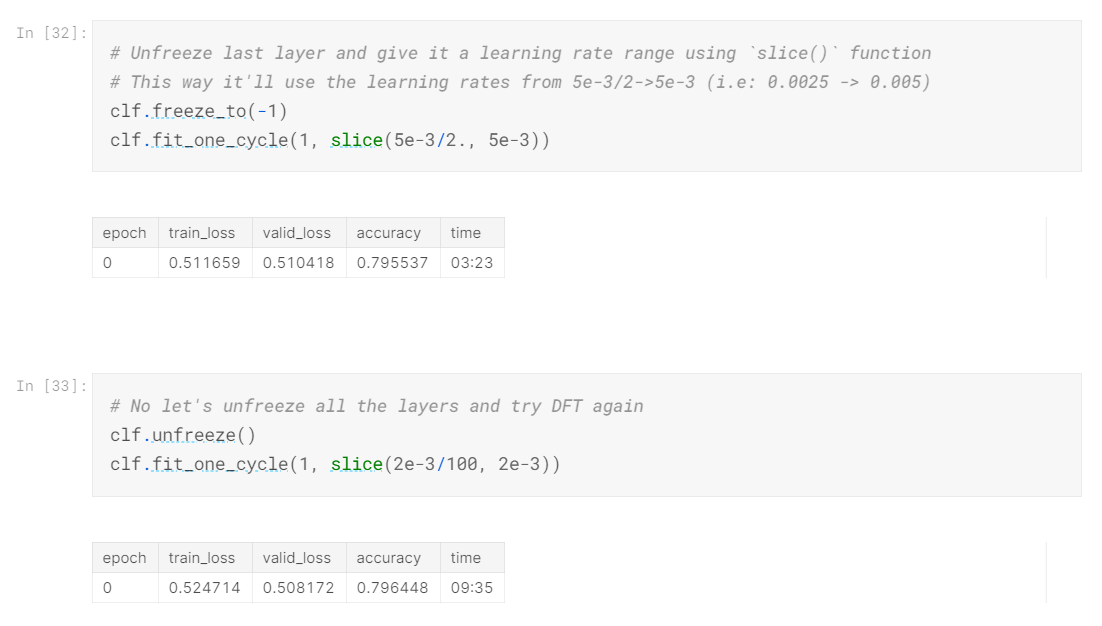
So at the end, we have achieved a final accuracy of ~80%.

Testing

Let’s now test our classifier on some strings.

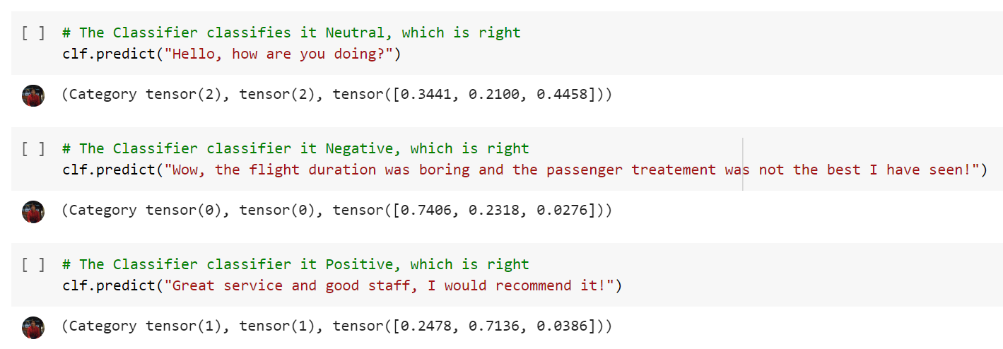
Remember that we have encoded our labels into (0,1,2), which is the reason why it’s prediction “Tensor(1)”, etc.

Conclusion

Huh, You’ve made it this far! Thank you for taking some time out of your schedule for reading my blogpost!

Please pardon and correct me if I’ve made any mistakes in EDA, modelling or maybe explaining some concept since I am a beginner and prone to making mistakes.

–Tanay Mehta

---